What are decision boundaries ?
Quoting Wikipedia:
In a statistical-classification problem with two classes, a decision boundary or decision surface is a hypersurface that partitions the underlying vector space into two sets, one for each class. The classifier will classify all the points on one side of the decision boundary as belonging to one class and all those on the other side as belonging to the other class.
Put another way, points on the decision boundary are the point for which the classifier cannot tell which class they belong to.
Why are decision boundaries important
Apart from being a quite common question in data science job interviews, they may help to understand other topics, such as having an insight on what algorithm may work on your data (though that is only true for datasets with a small dimension) or having an intuition on why blending works (see my other article theory behind model stacking for more information about this).
Decision boundary of a linear model
A straight line. No suprises, the function estimated is a linear function.
_Contour.png)
_Heatmap.png)
Decision boundary of a decision tree
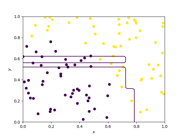
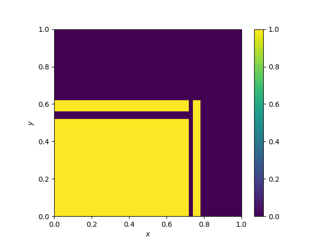
A decision tree follows a simple recursive splitting rule, where the splits, as they are performed according to one variable at a time are parallel to the axes. This is what we can observe below.
Decision boundary of Random Forests and extra trees
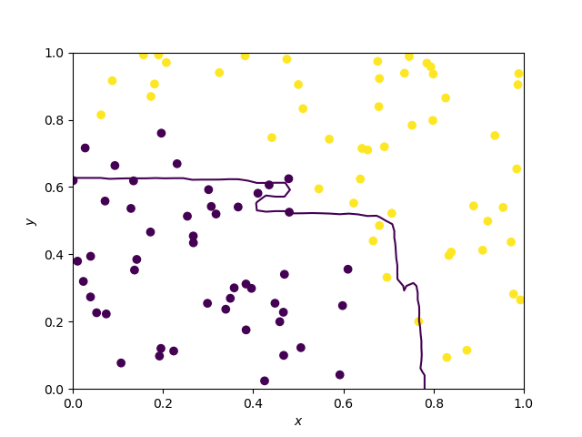
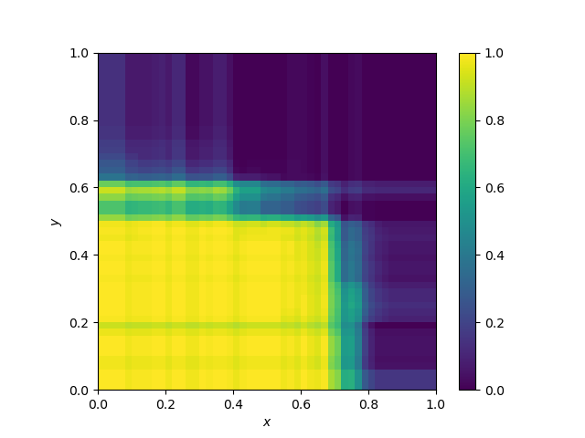
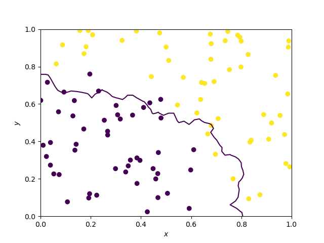
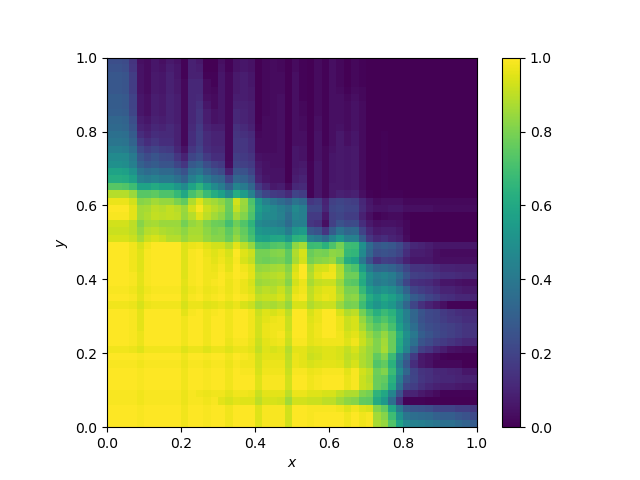
They are averages of decision trees borders and as such, they have a more general shape, but parallelism is still somehow visible. Note that the two decision boundaries are hard to dinstinguish.
Random forest
Extra trees
Decision boundary of KNN algorithms
When k, the number of neighbors to use to predict a new point is set to one, this represents a Voronoi diagram.
k=1
_Contour.png)
_Heatmap.png)
k=5
With k = 5 we start to have an estimation of the probability by counting the nearest neighbors in each class. Therefore, the decision boundary is “smoother”, than for k = 1.
_Contour.png)
_Heatmap.png)
Decision boundary of Support Vector Machines
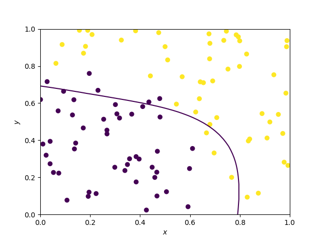
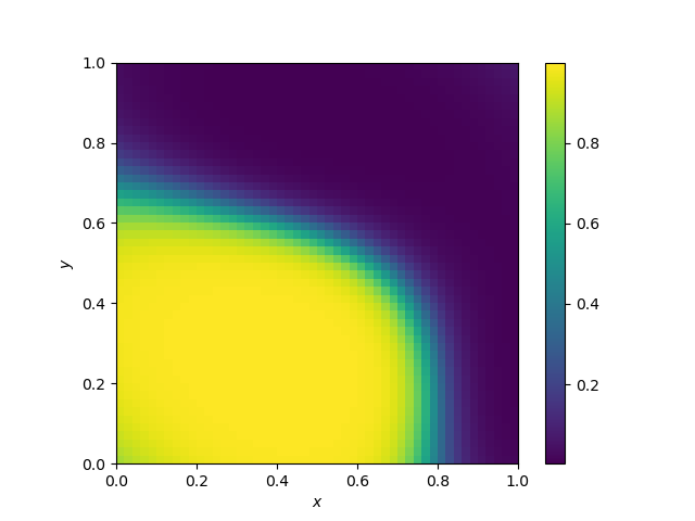
They should vary vastly on the kernel. Here, the kernel is gaussian.
The kernel below is the default SVC kernel (radial basis function, rbf):
Reproducing the results
I used the DecisionBoundaryPlotter that you may have seen in theory behind model stacking because writing machine learning scripts feels so much better when you reuse code ;)
import numpy as np
import matplotlib.pyplot as plt


class DecisionBoundaryPlotter:

    def __init__(self, X, Y, xs=np.linspace(0, 1, 50),
                 ys=np.linspace(0, 1, 50)):
        self._X = X
        self._Y = Y
        self._xs = xs
        self._ys = ys

    def _predictor(self, model):
        model.fit(self._X, self._Y)
        return (lambda x: model.predict_proba(x.reshape(1, -1))[0, 0])

    def _evaluate_height(self, f):
        fun_map = np.empty((self._xs.size, self._ys.size))
        for i in range(self._xs.size):
            for j in range(self._ys.size):
                v = f(
                    np.array([self._xs[i], self._ys[j]]))
                fun_map[i, j] = v
        return fun_map

    def plot_heatmap(self, model, name):
        f = self._predictor(model)
        fun_map = self._evaluate_height(f)

        fig = plt.figure()
        s = fig.add_subplot(1, 1, 1, xlabel='$x$', ylabel='$y$')
        im = s.imshow(
            fun_map,
            extent=(self._ys[0], self._ys[-1], self._xs[0], self._xs[-1]),
            origin='lower')
        fig.colorbar(im)
        fig.savefig(name + '_Heatmap.png')

    def plot_contour(self, model, name):
        f = self._predictor(model)
        fun_map = self._evaluate_height(f)

        fig = plt.figure()
        s = fig.add_subplot(1, 1, 1, xlabel='$x$', ylabel='$y$')
        s.contour(self._xs, self._ys, fun_map, levels=[0.5])
        s.scatter(self._X[:, 0], self._X[:, 1], c=self._Y)
        fig.savefig(name + '_Contour.png')


if __name__ == "__main__":
    import numpy as np
    from sklearn.ensemble import RandomForestClassifier, ExtraTreesClassifier, AdaBoostClassifier
    from sklearn.tree import DecisionTreeClassifier
    from sklearn.svm import SVR, SVC
    from sklearn.neighbors import KNeighborsClassifier
    from sklearn.linear_model import LogisticRegression

    def random_data_classification(n, p, f):
        predictors = np.random.rand(n, p)
        return predictors, np.apply_along_axis(f, 1, predictors)

    def parabolic(x, y):
        return (x**2 + y**3 > 0.5) * 1

    def parabolic_mat(x):
        return parabolic(x[0], x[1])

    X, Y = random_data_classification(100, 2, parabolic_mat)

    dbp = DecisionBoundaryPlotter(X, Y)

    named_classifiers = [(RandomForestClassifier(), "RandomForestClassifier"),
                         (ExtraTreesClassifier(), "ExtraTreesClassifier"),
                         (DecisionTreeClassifier(max_depth=4), "DecisionTreeClassifier"),
                         (AdaBoostClassifier(), "AdaBoostClassifier"),
                         (KNeighborsClassifier(n_neighbors=5), "KNN(5)"),
                         (KNeighborsClassifier(n_neighbors=1), "KNN(1)"),
                         (SVC(probability=True), "SVC"),
                         (LogisticRegression(), "LogisticRegression(solver=liblinear)")]

    for named_classifier in named_classifiers:
        print(named_classifier[1])
        dbp.plot_contour(named_classifier[0], named_classifier[1])
        dbp.plot_heatmap(named_classifier[0], named_classifier[1])
